Writing Raster Data

RasterFrames is oriented toward large scale analyses of spatial data. The primary output of these analyses could be a statistical summary, a machine learning model, or some other result that is generally much smaller than the input dataset.

However, there are times in any analysis where writing a representative sample of the work in progress provides valuable feedback on the current state of the process and results, or you are constructing a new dataset to be used in other analyses.

This will be our setup for the following examples:

from pyrasterframes import *
from pyrasterframes.rasterfunctions import *
from pyrasterframes.utils import create_rf_spark_session
import pyrasterframes.rf_ipython
from IPython.display import display
import os.path
spark = create_rf_spark_session(**{
    'spark.driver.memory': '4G',
    'spark.ui.enabled': 'false'
})
def scene(band):
    b = str(band).zfill(2) # converts int 2 to '02'
    return 'https://modis-pds.s3.amazonaws.com/MCD43A4.006/11/08/2019059/' \
             'MCD43A4.A2019059.h11v08.006.2019072203257_B{}.TIF'.format(b)
rf = spark.read.raster(scene(2), tile_dimensions=(256, 256))

IPython/Jupyter

This section provides details on how Tiles and DataFrames with Tiles in them can be viewed in the IPython/Jupyter.

Overview Rasters

In cases where writing and reading to/from a GeoTIFF isn’t convenient, RasterFrames provides the rf_agg_overview_raster aggregate function, where you can construct a single raster (rendered as a tile) downsampled from all or a subset of the DataFrame. This allows you to effectively construct the same operations the GeoTIFF writer performs, but without the file I/O.

The rf_agg_overview_raster function will reproject data to the commonly used “web mercator” CRS. You must specify an “Area of Interest” (AOI) in web mercator. You can use rf_agg_reprojected_extent to compute the extent of a DataFrame in any CRS or mix of CRSs.

wm_extent = rf.agg(
                  rf_agg_reprojected_extent(rf_extent('proj_raster'), rf_crs('proj_raster'), 'EPSG:3857')
                  ).first()[0]
aoi = Extent.from_row(wm_extent)
print(aoi)
aspect = aoi.width / aoi.height

ov = rf.agg(
    rf_agg_overview_raster('proj_raster', int(512 * aspect), 512, aoi)
).first()[0]
print("`ov` is of type", type(ov))
ov

Extent(-7912574.135382183, -7.081154551613622E-10, -6679169.446996604, 1118889.9747567875)
`ov` is of type <class 'pyrasterframes.rf_types.Tile'>

GeoTIFFs

GeoTIFF is one of the most common file formats for spatial data, providing flexibility in data encoding, representation, and storage. RasterFrames provides a specialized Spark DataFrame writer for rendering a RasterFrame to a GeoTIFF. It is accessed by calling dataframe.write.geotiff.

Limitations and mitigations

One downside to GeoTIFF is that it is not a big-data native format. To create a GeoTIFF, all the data to be written must be collected in the memory of the Spark driver. This means you must actively limit the size of the data to be written. It is trivial to lazily read a set of inputs that cannot feasibly be written to GeoTIFF in the same environment.

When writing GeoTIFFs in RasterFrames, you should limit the size of the collected data. Consider filtering the dataframe by time or spatial filters.

You can also specify the dimensions of the GeoTIFF file to be written using the raster_dimensions parameter as described below.

Parameters

If there are many tile or projected raster columns in the DataFrame, the GeoTIFF writer will write each one as a separate band in the file. Each band in the output will be tagged the input column names for reference.

• path: the path local to the driver where the file will be written
• crs: the PROJ4 string of the CRS the GeoTIFF is to be written in
• raster_dimensions: optional, a tuple of two ints giving the size of the resulting file. If specified, RasterFrames will downsample the data in distributed fashion using bilinear resampling. If not specified, the default is to write the dataframe at full resolution, which can result in an out of memory error.

Example

See also the example in the unsupervised learning page.

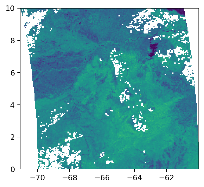
Let’s render an overview of a scene’s red band as a small raster, reprojecting it to latitude and longitude coordinates on the WGS84 reference ellipsoid (aka EPSG:4326).

outfile = os.path.join('/tmp', 'geotiff-overview.tif')
rf.write.geotiff(outfile, crs='EPSG:4326', raster_dimensions=(256, 256))

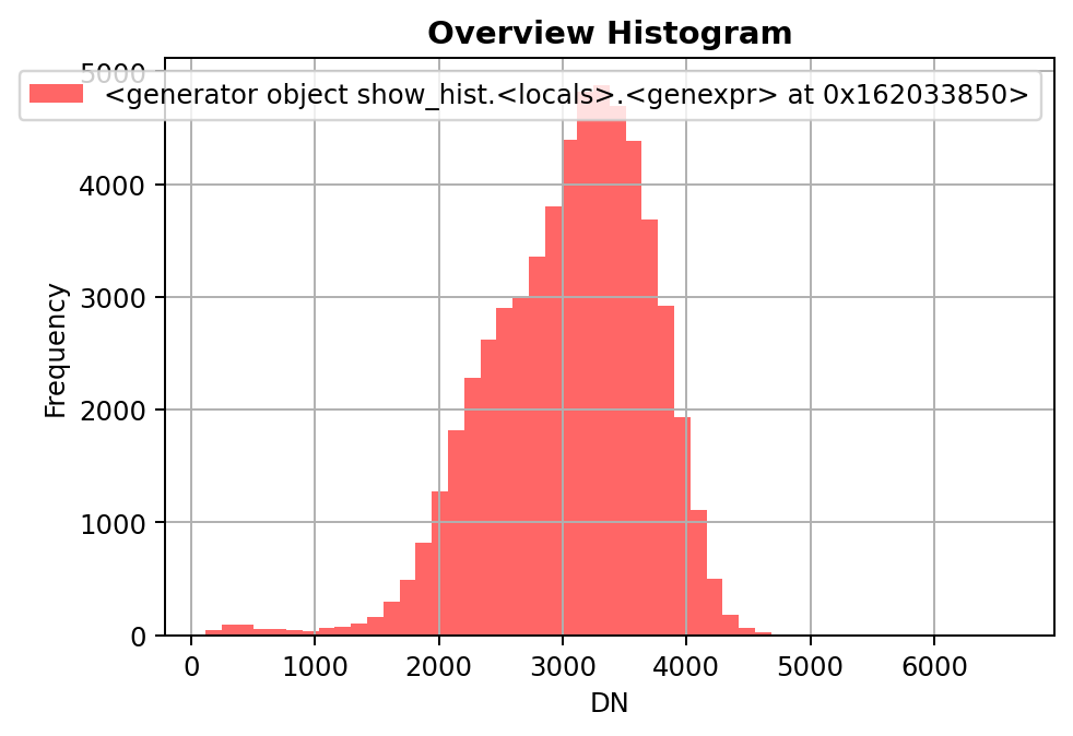
We can view the written file with rasterio:

import rasterio
from rasterio.plot import show, show_hist

with rasterio.open(outfile) as src:
    # View raster
    show(src, adjust='linear')
    # View data distribution
    show_hist(src, bins=50, lw=0.0, stacked=False, alpha=0.6,
        histtype='stepfilled', title="Overview Histogram")

Color Composites

If the DataFrame has three or four tile columns, the GeoTIFF is written with the ColorInterp tags on the bands to indicate red, green, blue, and optionally alpha. Use a select statement to ensure the bands are in the desired order. If the bands chosen are red, green, and blue, the composite is called a true-color composite. Otherwise it is a false-color composite. If the number of tile columns is not 3 or 4, the ColorInterp tag will indicate greyscale.

Also see Color Composite in the IPython/Juptyer Extensions.

PNG

In this example we will use the rf_rgb_composite function, we will compute a three band PNG image as a bytearray. The resulting bytearray will be displayed as an image in either a Spark or pandas DataFrame display if rf_ipython has been imported.

# Select red, green, and blue, respectively
composite_df = spark.read.raster([[scene(1), scene(4), scene(3)]])

composite_df = composite_df.withColumn('png',
                    rf_render_png('proj_raster_0', 'proj_raster_1', 'proj_raster_2')).cache()
composite_df.select('png').limit(1)

png

Alternatively the bytearray result can be displayed with pillow.

import io
from PIL.Image import open as PIL_open
png_bytearray = composite_df.first()['png']
pil_image = PIL_open(io.BytesIO(png_bytearray))
pil_image

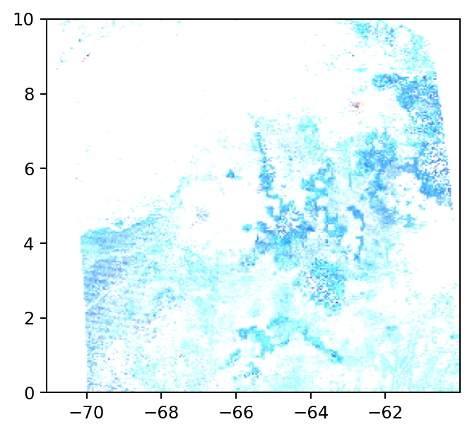
GeoTIFF

In this example we will write a false-color composite as a GeoTIFF

outfile = os.path.join('/tmp', 'geotiff-composite.tif')
composite_df = spark.read.raster([[scene(3), scene(1), scene(4)]])
composite_df.write.geotiff(outfile, crs='EPSG:4326', raster_dimensions=(256, 256))

with rasterio.open(outfile) as src:
    show(src)

GeoTrellis Layers

GeoTrellis is one of the key libraries upon which RasterFrames is built. It provides a Scala language API for working with geospatial raster data. GeoTrellis defines a tile layer storage format for persisting imagery mosaics. RasterFrames can write data from a RasterFrameLayer into a GeoTrellis Layer. RasterFrames provides a geotrellis DataSource that supports both reading and writing GeoTrellis layers.

An example is forthcoming. In the mean time referencing the GeoTrellisDataSourceSpec test code may help.

Parquet

You can write a RasterFrame to the Apache Parquet format. This format is designed to efficiently persist and query columnar data in distributed file system, such as HDFS. It also provides benefits when working in single node (or “local”) mode, such as tailoring organization for defined query patterns.

rf.withColumn('exp', rf_expm1('proj_raster')) \
    .write.mode('append').parquet('hdfs:///rf-user/sample.pq')