Local Map Algebra
Local map algebra raster operations are element-wise operations on a single tile, between a tile and a scalar, between two tiles, or among many tiles. These operations are common in processing of earth observation imagery and other image data.
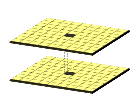
Credit: GISGeography
Computing NDVI
Here is an example of computing the Normalized Differential Vegetation Index (NDVI). NDVI is a vegetation index which emphasizes differences in relative biomass and vegetation health. The term index in Earth observation means a combination of many raster bands into a single band that highlights a phenomenon of interest. Various indices have proven useful visual tools and frequently appear as features in machine learning models using Earth observation data.
NDVI is often used worldwide to monitor drought, monitor and predict agricultural production, assist in predicting hazardous fire zones, and map desert encroachment. The NDVI is preferred for global vegetation monitoring because it helps to compensate for changing illumination conditions, surface slope, aspect, and other extraneous factors (Lillesand. Remote sensing and image interpretation. 2004)
We will apply the catalog pattern for defining the data we wish to process. To compute NDVI we need to compute local algebra on the red and near infrared (nir) bands:
       nir - red
NDVI = ---------
       nir + red
This form of (x - y) / (x + y) is common in remote sensing and is called a normalized difference. It is used with other band pairs to highlight water, snow, and other phenomena.
from pyspark.sql import Row
uri_pattern = 'https://rasterframes.s3.amazonaws.com/samples/luray_snp/B0{}.tif'
catalog_df = spark.createDataFrame([
    Row(red=uri_pattern.format(4), nir=uri_pattern.format(8))
])
df = spark.read.raster(
    catalog_df,
    catalog_col_names=['red', 'nir']
)
df.printSchema()
root
 |-- red_path: string (nullable = false)
 |-- nir_path: string (nullable = false)
 |-- red: struct (nullable = true)
 |    |-- tile_context: struct (nullable = true)
 |    |    |-- extent: struct (nullable = false)
 |    |    |    |-- xmin: double (nullable = false)
 |    |    |    |-- ymin: double (nullable = false)
 |    |    |    |-- xmax: double (nullable = false)
 |    |    |    |-- ymax: double (nullable = false)
 |    |    |-- crs: struct (nullable = false)
 |    |    |    |-- crsProj4: string (nullable = false)
 |    |-- tile: tile (nullable = false)
 |-- nir: struct (nullable = true)
 |    |-- tile_context: struct (nullable = true)
 |    |    |-- extent: struct (nullable = false)
 |    |    |    |-- xmin: double (nullable = false)
 |    |    |    |-- ymin: double (nullable = false)
 |    |    |    |-- xmax: double (nullable = false)
 |    |    |    |-- ymax: double (nullable = false)
 |    |    |-- crs: struct (nullable = false)
 |    |    |    |-- crsProj4: string (nullable = false)
 |    |-- tile: tile (nullable = false)
Observe how the bands we need to use to compute the index are arranged as columns of our resulting DataFrame. The rows or observations are various spatial extents within the entire coverage area.
RasterFrames provides a wide variety of local map algebra functions. There are several different broad categories, based on how many tiles the function takes as input:
- A function on a single tile is a unary operation; example: rf_log;
- A function on two tiles is a binary operation; example: rf_local_multiply;
- A function on a tile and a scalar is a binary operation; example: rf_local_less; or
- A function on many tiles is a n-ary operation; example: rf_agg_local_min
We can express the normalized difference with a combination of rf_local_divide, rf_local_subtract, and rf_local_add. Since the normalized difference is so common, there is a convenience method rf_normalized_difference, which we use in this example. We will append a new column to the DataFrame, which will apply the map alegbra function to each row.
df = df.withColumn('ndvi', rf_normalized_difference(df.nir, df.red))
df.printSchema()
root
 |-- red_path: string (nullable = false)
 |-- nir_path: string (nullable = false)
 |-- red: struct (nullable = true)
 |    |-- tile_context: struct (nullable = true)
 |    |    |-- extent: struct (nullable = false)
 |    |    |    |-- xmin: double (nullable = false)
 |    |    |    |-- ymin: double (nullable = false)
 |    |    |    |-- xmax: double (nullable = false)
 |    |    |    |-- ymax: double (nullable = false)
 |    |    |-- crs: struct (nullable = false)
 |    |    |    |-- crsProj4: string (nullable = false)
 |    |-- tile: tile (nullable = false)
 |-- nir: struct (nullable = true)
 |    |-- tile_context: struct (nullable = true)
 |    |    |-- extent: struct (nullable = false)
 |    |    |    |-- xmin: double (nullable = false)
 |    |    |    |-- ymin: double (nullable = false)
 |    |    |    |-- xmax: double (nullable = false)
 |    |    |    |-- ymax: double (nullable = false)
 |    |    |-- crs: struct (nullable = false)
 |    |    |    |-- crsProj4: string (nullable = false)
 |    |-- tile: tile (nullable = false)
 |-- ndvi: struct (nullable = true)
 |    |-- tile_context: struct (nullable = true)
 |    |    |-- extent: struct (nullable = false)
 |    |    |    |-- xmin: double (nullable = false)
 |    |    |    |-- ymin: double (nullable = false)
 |    |    |    |-- xmax: double (nullable = false)
 |    |    |    |-- ymax: double (nullable = false)
 |    |    |-- crs: struct (nullable = false)
 |    |    |    |-- crsProj4: string (nullable = false)
 |    |-- tile: tile (nullable = false)
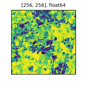
We can inspect a sample of the data. Yellow indicates very healthy vegetation, and purple represents bare soil or impervious surfaces.
t = df.select(rf_tile('ndvi').alias('ndvi')).first()['ndvi']
display(t)

We continue examining NDVI in the time series section.