Masking
Masking is a common operation in raster processing. It is setting certain cells to the NoData value. This is usually done to remove low-quality observations from the raster processing. Another related use case is to “clip” a raster to a given polygon.
In this section we will demonstrate two common schemes for masking. In Sentinel 2, there is a separate classification raster that defines low quality areas. In Landsat 8, several quality factors are measured and the indications are packed into a single integer, which we have to unpack.
Masking Sentinel 2
Let’s demonstrate masking with a pair of bands of Sentinel-2 data. The measurement bands we will use, blue and green, have no defined NoData. They share quality information from a separate file called the scene classification (SCL), which delineates areas of missing data and probable clouds. For more information on this, see the Sentinel-2 algorithm overview. Figure 3 tells us how to interpret the scene classification. For this example, we will exclude NoData, defective pixels, probable clouds, and cirrus clouds: values 0, 1, 8, 9, and 10.
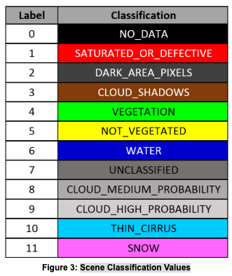
Credit: Sentinel-2 algorithm overview
The first step is to create a catalog with our band of interest and the SCL band. We read the data from the catalog, so all tiles are aligned across rows.
from pyspark.sql import Row

blue_uri = 'https://rasterframes.s3.amazonaws.com/samples/luray_snp/B02.tif'
green_uri = 'https://rasterframes.s3.amazonaws.com/samples/luray_snp/B03.tif'
scl_uri = 'https://rasterframes.s3.amazonaws.com/samples/luray_snp/SCL.tif'
cat = spark.createDataFrame([Row(blue=blue_uri, green=green_uri, scl=scl_uri),])
unmasked = spark.read.raster(cat, catalog_col_names=['blue', 'green', 'scl'])
unmasked.printSchema()
root
 |-- blue_path: string (nullable = false)
 |-- green_path: string (nullable = false)
 |-- scl_path: string (nullable = false)
 |-- blue: struct (nullable = true)
 |    |-- tile_context: struct (nullable = true)
 |    |    |-- extent: struct (nullable = false)
 |    |    |    |-- xmin: double (nullable = false)
 |    |    |    |-- ymin: double (nullable = false)
 |    |    |    |-- xmax: double (nullable = false)
 |    |    |    |-- ymax: double (nullable = false)
 |    |    |-- crs: struct (nullable = false)
 |    |    |    |-- crsProj4: string (nullable = false)
 |    |-- tile: tile (nullable = false)
 |-- green: struct (nullable = true)
 |    |-- tile_context: struct (nullable = true)
 |    |    |-- extent: struct (nullable = false)
 |    |    |    |-- xmin: double (nullable = false)
 |    |    |    |-- ymin: double (nullable = false)
 |    |    |    |-- xmax: double (nullable = false)
 |    |    |    |-- ymax: double (nullable = false)
 |    |    |-- crs: struct (nullable = false)
 |    |    |    |-- crsProj4: string (nullable = false)
 |    |-- tile: tile (nullable = false)
 |-- scl: struct (nullable = true)
 |    |-- tile_context: struct (nullable = true)
 |    |    |-- extent: struct (nullable = false)
 |    |    |    |-- xmin: double (nullable = false)
 |    |    |    |-- ymin: double (nullable = false)
 |    |    |    |-- xmax: double (nullable = false)
 |    |    |    |-- ymax: double (nullable = false)
 |    |    |-- crs: struct (nullable = false)
 |    |    |    |-- crsProj4: string (nullable = false)
 |    |-- tile: tile (nullable = false)
unmasked.select(rf_cell_type('blue'), rf_cell_type('scl')).distinct()
| rf_cell_type(blue) | rf_cell_type(scl) |
|---|---|
| [uint16raw] | [uint8raw] |
Define CellType for Masked Tile
Because there is not a NoData already defined for the blue band, we must choose one. If we try to apply a masking function to a tile whose cell type has no NoData defined, an error will be thrown.
In this particular example, the minimum value of all cells in all tiles in the column is greater than zero, so we can use 0 as the NoData value. We will construct a new CellType object to represent this.
blue_min = unmasked.agg(rf_agg_stats('blue').min.alias('blue_min'))
print('Nonzero minimum value in the blue band:', blue_min.first())

blue_ct = unmasked.select(rf_cell_type('blue')).distinct().first()[0][0]
masked_blue_ct = CellType(blue_ct).with_no_data_value(0)
masked_blue_ct.cell_type_name
Nonzero minimum value in the blue band: Row(blue_min=3.0)
'uint16ud0'
We next convert the blue band to this cell type.
converted = unmasked.select('scl', 'green', rf_convert_cell_type('blue', masked_blue_ct).alias('blue'))
Apply Mask from Quality Band
Now we set cells of our blue column to NoData for all locations where the scl tile is in our set of undesirable values. This is the actual masking operation.
from pyspark.sql.functions import lit

masked = converted.withColumn('blue_masked', rf_mask_by_values('blue', 'scl', [0, 1, 8, 9, 10]))
masked
Showing only top 5 rows.
| scl | green | blue | blue_masked |
|---|---|---|---|
 |
 |
 |
 |
 |
 |
 |
 |
 |
 |
 |
 |
 |
 |
 |
|
 |
 |
 |
 |
We can verify that the number of NoData cells in the resulting blue_masked column matches the total of the boolean mask tile to ensure our logic is correct.
masked.select(rf_no_data_cells('blue_masked'), rf_tile_sum(rf_local_is_in('scl', [0, 1, 8, 9, 10])))
Showing only top 5 rows.
| rf_no_data_cells(blue_masked) | rf_tile_sum(rf_local_is_in(scl, array(0, 1, 8, 9, 10))) |
|---|---|
| 247 | 247.0 |
| 16 | 16.0 |
| 131 | 131.0 |
| 0 | 0.0 |
| 5 | 5.0 |
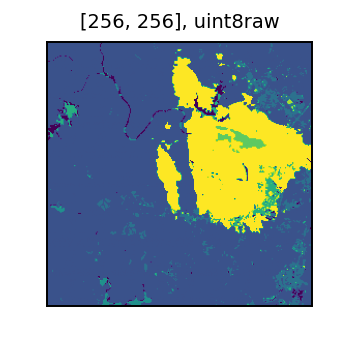
It’s also nice to view a sample. The white regions are areas of NoData.
sample = masked.orderBy(-rf_no_data_cells('blue_masked')).select(rf_tile('blue_masked'), rf_tile('scl')).first()
display(sample[0])

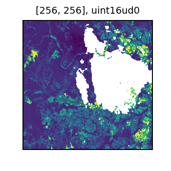
And the original SCL data. The bright yellow is a cloudy region in the original image.
display(sample[1])

Transferring Mask
We can now apply the same mask from the blue column to the green column. Note here we have supressed the step of explicitly checking what a “safe” NoData value for the green band should be.
masked.withColumn('green_masked', rf_mask(rf_convert_cell_type('green', masked_blue_ct), 'blue_masked'))  \
      .orderBy(-rf_no_data_cells('blue_masked'))
Showing only top 5 rows.
| scl | green | blue | blue_masked | green_masked |
|---|---|---|---|---|
 |
 |
 |
 |
 |
 |
 |
 |
 |
 |
 |
 |
 |
 |
 |
 |
 |
 |
 |
 |
 |
 |
 |
 |
 |
Masking Landsat 8
We will work with the Landsat scene here. For simplicity, we will just use two of the seven 30m bands. The quality mask for all bands is all contained in the BQA band.
base_url = 'https://landsat-pds.s3.us-west-2.amazonaws.com/c1/L8/153/075/LC08_L1TP_153075_20190718_20190731_01_T1/LC08_L1TP_153075_20190718_20190731_01_T1_'
data4 = base_url + 'B4.TIF'
data2 = base_url + 'B2.TIF'
mask = base_url + 'BQA.TIF'
l8_df = spark.read.raster([[data4, data2, mask]]) \
               .withColumnRenamed('proj_raster_0', 'data') \
               .withColumnRenamed('proj_raster_1', 'data2') \
               .withColumnRenamed('proj_raster_2', 'mask')
Masking is described on the Landsat Missions page. It is pretty dense. Focus for this data set is the Collection 1 Level-1 for Landsat 8.
There are several inter-related factors to consider. In this exercise we will mask away the following.
- Designated Fill = yes
- Cloud = yes
- Cloud Shadow Confidence = Medium or High
- Cirrus Confidence = Medium or High
Note that you should consider your application and do your own exploratory analysis to determine the most appropriate mask!
According to the information on the Landsat site this translates to masking by bit values in the BQA according to the following table.
| Description | Value | Bits | Bit values |
|---|---|---|---|
| Designated fill | yes | 0 | 1 |
| Cloud | yes | 4 | 1 |
| Cloud shadow conf. | med / hi | 7-8 | 10, 11 (2, 3) |
| Cirrus conf. | med / hi | 11-12 | 10, 11 (2, 3) |
In this case, we will use the value of 0 as the NoData in the band data. Inspecting the associated MTL txt file By inspection, we can discover that the minimum value in the band will be 1, thus allowing our use of 0 for NoData.
The code chunk below works through each of the rows in the table above. The first expression sets the cell type to have the selected NoData. The rf_mask_by_bit and rf_mask_by_bits functions extract the selected bit or bits from the mask cells and compare them to the provided values.
l8_df = l8_df.withColumn('data_masked', # set to cell type that has a nodata
                   rf_convert_cell_type('data', CellType.uint16())) \
       .withColumn('data_masked', # fill yes
                  rf_mask_by_bit('data_masked', 'mask', 0, 1)) \
       .withColumn('data_masked', # cloud yes
                  rf_mask_by_bit('data_masked', 'mask', 4, 1)) \
       .withColumn('data_masked', # cloud shadow conf is medium or high
                  rf_mask_by_bits('data_masked', 'mask', 7, 2, [2, 3])) \
       .withColumn('data_masked', # cloud shadow conf is medium or high
                  rf_mask_by_bits('data_masked', 'mask', 11, 2, [2, 3])) \
       .withColumn('data2', # mask other data col against the other band
                  rf_mask(rf_convert_cell_type('data2',CellType.uint16()), 'data_masked')) \
       .filter(rf_data_cells('data_masked') > 0) # remove any entirely ND rows

# Inspect a sample
l8_df.select('data', 'mask', 'data_masked', 'data2', rf_extent('data_masked')) \
     .filter(rf_data_cells('data_masked') > 32000)
Showing only top 5 rows.
| data | mask | data_masked | data2 | rf_extent(data_masked) |
|---|---|---|---|---|
 |
 |
 |
 |
[363525.0, -2327565.0, 371205.0, -2319885.0] |
 |
 |
 |
 |
[355845.0, -2488845.0, 363525.0, -2481165.0] |
 |
 |
 |
 |
[286725.0, -2450445.0, 294405.0, -2442765.0] |
 |
 |
 |
 |
[432645.0, -2419725.0, 440325.0, -2412045.0] |
 |
 |
 |
 |
[378885.0, -2381325.0, 386565.0, -2373645.0] |
Clipping
Clipping is the use of a polygon to determine the areas to mask in a raster. Typically the areas inside a polygon are retained and the cells outside are set to NoData. Given a geometry column on our DataFrame, we have to carry out three basic steps. First we have to ensure the vector geometry is correctly projected to the same CRS as the raster. We’ll continue with our Sentinel 2 example, creating a simple polygon. Buffering a point will create an approximate circle.
to_rasterize = masked.withColumn('geom_4326',
                            st_bufferPoint(
                                st_point(lit(-78.0783132), lit(38.3184340)),
                                lit(15000))) \
                .withColumn('geom_native', st_reproject('geom_4326', rf_mk_crs('epsg:4326'), rf_crs('blue_masked')))
Second, we will rasterize the geometry, or burn-in the geometry into the same grid as the raster.
to_clip = to_rasterize.withColumn('clip_raster',
                                 rf_rasterize('geom_native', rf_geometry('blue_masked'), lit(1), rf_dimensions('blue_masked').cols, rf_dimensions('blue_masked').rows))

# visualize some of the edges of our circle
to_clip.select('blue_masked', 'clip_raster') \
    .filter(rf_data_cells('clip_raster') > 20) \
    .orderBy(rf_data_cells('clip_raster'))
Showing only top 5 rows.
| blue_masked | clip_raster |
|---|---|
 |
 |
 |
 |
 |
 |
 |
 |
 |
 |
Finally, we create a new tile column with the blue band clipped to our circle. Again we will use the rf_mask function to pass the NoData regions along from the rasterized geometry.
to_clip.select('blue_masked',
               'clip_raster',
               rf_mask('blue_masked', 'clip_raster').alias('blue_clipped')) \
           .filter(rf_data_cells('clip_raster') > 20) \
           .orderBy(rf_data_cells('clip_raster'))
Showing only top 5 rows.
| blue_masked | clip_raster | blue_clipped |
|---|---|---|
| |
|
 |
| |
|
 |
| |
|
 |
| |
|
 |
| |
|
 |
This kind of clipping technique is further used in zonal statistics.